IQ Data Compression Techniques for Bandwidth-Constrained Open Fronthaul

1. Introduction & Structural Background

The transition from traditional monolithic Base Stations to disaggregated Open Radio Access Networks (O-RAN) has fundamentally reshaped the telecommunications industry. In a classic Distributed RAN (D-RAN), the baseband processing and RF frontends are tightly integrated using proprietary point-to-point protocols like the Common Public Radio Interface (CPRI). CPRI transmits continuous time-domain, uncompressed In-phase and Quadrature (IQ) waveforms. While this maintains optimal signal fidelity, it scales linearly with carrier bandwidth, sampling rate, and the number of antenna elements. For modern 5G architectures utilizing Massive MIMO (mMIMO) and wide frequency bands, raw time-domain CPRI transport data rates can easily exceed several Terabits per second per tower—making dedicated optical fiber links prohibitively expensive.

To solve this scaling problem, the O-RAN Alliance standardized the Functional Split 7.2x for the Lower Layer Split (LLS) between the Open Distributed Unit (O-DU) and the Open Radio Unit (O-RU). Split 7.2x moves the Fast Fourier Transform (FFT) and Inverse Fast Fourier Transform (IFFT) functions into the O-RU. Consequently, instead of continuous time-domain noise and waveforms, the open fronthaul interface transports data in the frequency domain as subcarrier Resource Elements (REs) organized into Physical Resource Blocks (PRBs).     

Even with the data-rate reductions provided by the 7.2x frequency-domain split, wideband allocations—such as 100 MHz bands with a high number of antenna spatial layers—still place severe demands on packet-switched Ethernet fronthaul networks. This makes IQ Data Compression a crucial feature within the standard. By applying digital bit-reduction algorithms to the frequency-domain IQ symbols before packet encapsulation, networks can safely suppress data traffic. This approach prevents Ethernet link congestion and significantly reduces infrastructure deployment costs.

2. Why IQ Compression is Mandatory in Open Fronthaul

To understand why real-time compression is necessary, we must analyze the math behind uncompressed frequency-domain data generation. In a standard 5G New Radio (5G-NR) cell configuration using Split 7.2x, the uncompressed line rate is directly governed by several network parameters:

Where:

• 2 represents the two independent In-phase (I) and Quadrature (Q) components per complex sample.

• Wraw is the raw quantization bit-width (typically 16 bits per component in uncompressed baseband engines).

• Nsc is the number of active subcarriers across the system bandwidth.

• Nsym is the number of OFDM symbols generated per second.

• Nlayers is the total number of simultaneous antenna spatial streams (MIMO layers).

For an uncompressed 100 MHz TDD carrier with a 30 kHz Subcarrier Spacing (SCS), the system yields 273 active PRBs (3,276 subcarriers) operating across 14 OFDM symbols every 0.5 milliseconds (28,000 symbols per second). In a 4T4R spatial layout, the continuous bit rate reaches:

When scaling up to a 64T64R Massive MIMO array under high traffic configurations, the required bandwidth expands to over 188 Gbps for a single sector. If an operator plans to co-locate three sectors on a single hub site, the required backhaul bandwidth approaches 564 Gbps.

Standard commercial transport infrastructures rely primarily on 100G or 25G Ethernet transport links. Forcing uncompressed streams onto these links causes severe packet drops, increased transmission delays, and strict queue blockages. IQ compression acts as an optimized, real-time bit-reduction step. It condenses wide-bit integer streams into narrow bit envelopes, fitting multi-layer sectors into standard, cost-effective fiber links.

3. Core Compression Algorithms: Mechanisms and Examples

The O-RAN Alliance specifies three primary mathematical compression methods to balance computing complexity against signal fidelity:

1. Block Floating Point (BFP)

2. Block Scaling (BS)

3. u law Companding

3.1 Block Floating Point (BFP) Compression

Block Floating Point is the most widely adopted algorithm in commercial O-RAN deployments due to its excellent performance and low hardware overhead. BFP operates on a block of samples—typically a single Physical Resource Block (PRB) containing 12 complex IQ resource elements.

Mathematical Mechanism

The algorithm looks at all 24 integer values within a PRB(12x I, 12x Q) and determines the single largest absolute peak value. It determines the number of bits required to represent this peak value without clipping. This value becomes the shared "Exponent" (E) for the entire block. Every sample in the block is then bit-shifted to match this exponent, discarding redundant sign bits or unneeded low-order bits. The truncated values are packed into a target bit-width Wtarget

Step-by-Step Example

Consider a simplified block containing three raw 16-bit IQ samples (I, Q pair integers):

Sample 1: I1 = 3400, Q1 = -512

Sample 2: I2 = 120, Q2 = 4100

Sample 3: I3 = -250, Q3 = 15

1. Find Peak Magnitude: The largest value in the block is Q2 = 4100.

2. Calculate Exponent: Representing +/-4100 in signed binary requires 14 bits (4100 falls between -8192 and +8191). The shared block exponent E is set to 14.

3. Calculate Mantissa Values or Compress to Target Width (Wtarget = 9 bits): The shift amount is calculated as S = E - Wtarget + 1 = 14 - 9 + 1 = 6 bits. Each value is right shifted by 6 bits (divided by 64) and rounded to the nearest integer.

4. Fronthaul Packet Structure: The single 8-bit exponent header (E=14) is sent once, followed immediately by the compressed 9-bit samples. This approach saves considerable link space compared to transmitting raw 16-bit integers.

   1. Raw Data Structure (Uncompressed PRB):

      [16-bit I1][16-bit Q1][16-bit I2][16-bit Q2] ... Total = 384 bits per PRB

   2. BFP Data Structure (Compressed PRB at 9-bit target):

      [8-bit Exponent][9-bit I1][9-bit Q1][9-bit I2][9-bit Q2] ... Total = 224 bits per PRB

When a compressed 5G/6G data packet arrives over the Open Fronthaul (via eCPRI over Ethernet) at the Open Radio Unit (O-RU), it cannot be immediately converted into analog radio waves. It must first pass through an IQ Decompression Engine inside the O-RU's FPGA or ASIC.

Decompression is the exact mathematical inverse of the compression process.

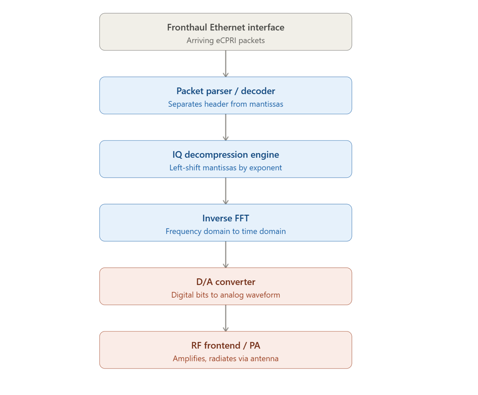
Step-by-Step Example of BFP Decompression

Let's assume the O-RU is configured for 9-bit BFP compression. The O-DU has compressed the data and sent it across the fiber link.

1. The Arriving Fronthaul Packet

The O-RU receives a data block representing a Physical Resource Block (PRB). The packet contains:

·       A shared Exponent Header (E): 14 (represented as an 8-bit integer: 00001110)

·       A stream of 9-bit compressed Mantissas (Icomp, Qcomp):

o   I1 = 53 (Binary: 000110101)

o   Q2 = 64 (Binary: 001000000)

2. The Decompression Formula

To restore the samples back to their original 16-bit linear baseline layout, the engine needs to know how many bits the O-DU originally shifted the data to the right.

The bit-shift value (S) is calculated using the target bit-width (Wtarget = 9) and the received exponent (E = 14):

S = E - Wtarget + 1 = 14 - 9 + 1 = 6 bits

The decompression engine reverses the compression by shifting the compressed mantissa left by S bits (which is mathematically equivalent to multiplying by 2^S or 2^6 = 64).

Idecomp = Icomp x 2^S

3. Executing the Reconstruction (The Hardware Shift)

Inside the O-RU's silicon fabric, a Barrel Shifter executes this left shift in a single clock cycle by appending zeros to the end of the binary string to pad it back out to 16 bits.

·       Reconstructing Sample I1:

o   Compressed value: 53 (000110101)

o   Shift Left by 6 bits: Multiply 53 x 64 = 3392

o   Resulting 16-bit signed integer: 3392

·       Reconstructing Sample Q_2:

o   Compressed value: 64 (001000000)

o   Shift Left by 6 bits: Multiply 64 x 64 = 4096

o   Resulting 16-bit signed integer: 4096

4. Comparing Raw vs. Decompressed Data

If we look back at the original uncompressed numbers before they were ever sent across the fronthaul:

·       Original I1 was 3400 -> Decompressed value is 3392 (Difference of -8)

·       Original Q2 was 4100 -> Decompressed value is 4096 (Difference of -4)

The tiny discrepancy between 3400 and 3392 is called quantization noise. Because a 9-bit mantissa cannot hold the ultra-fine resolution of the original lower 16-bit bits, those fine details are permanently lost during compression.

3.2 Block Scaling (BS) Compression

Block Scaling is structurally similar to BFP but operates in the linear domain using an explicit multiplication scaler rather than a binary bit-shift exponent.

Mathematical Mechanism

Instead of finding the nearest power-of-two exponent, Block Scaling calculates a floating-point master scaler value (Sblock) for the PRB. This scaler normalizes the maximum peak element to perfectly match the full dynamic range of the compressed target bit-width (Wtarget).

During decompression, the inverse scaler (1/Sblock) is multiplied back across the elements to reconstruct the original linear dynamic range.

Step-by-Step Example

Using a target compressed width of 9 bits (Wtarget = 9), the available signed integer dynamic range spans from -256 to +255.

1. Identify Maximum Absolute Value: Assume the peak value within the current PRB is 5000.

2. Compute Scaling Factor:

Sblock =  255/5000= 0.051

3. Compress the Samples: A sample with a raw value of I = 3200 is compressed using this linear scaling factor:

Icomp = 3200 * 0.051 =  floor(163.2)  = 163

4. Fronthaul Packet Structure: The calculated value 163 fits within the target 9-bit allocation. The master scaler block value (0.051) is quantized into an 8-bit side-information parameter and transmitted in the eCPRI application header.

3.3 u-law Companding

Derived from legacy PSTN voice architectures, u-law companding is a non-linear compression technique. It works well because wireless communications signals rarely maintain peak amplitudes; they spent most of their time at lower power levels.

Mathematical Mechanism

The u-law algorithm applies a logarithmic curve to the input signal before quantization. This process provides higher resolution (smaller step sizes) for low-amplitude signals and coarser resolution for large peaks. The standard O-RAN configuration sets the compression parameter u = 255.

Step-by-Step Example

1. Normalize Input: Scale the raw 16-bit integer to a fractional range between -1.0 and +1.0. Let a sample value of 2000 be normalized to x = 0.061.

2. Apply Logarithmic Transform:

   

3. Quantize to Target Width (e.g., 8 bits): Map the continuous value 0.506 onto an 8-bit signed integer range (-128 to +127):

Xcomp = 0.506  x127 ~= 64

Notice how a small input magnitude (0.061) maps to half the available output dynamic range (64). This logarithmic scaling keeps weak signals well above the quantization noise floor, though it can introduce distortion on high-amplitude peaks.

4. Hardware Implementation Architecture within the O-RU

Implementing compression within the O-RU requires an efficient hardware pipeline to process high-throughput data streams with minimal latency. The architectural pipeline must balance processing speed and hardware resource utilization inside an FPGA or ASIC.

4.1 The Compression Pipeline

The diagram below shows the processing stages inside an O-RU Uplink transmitter pipeline before data is sent across the open fronthaul interface:

4.2 BFP Implementation Block Diagram

Because Block Floating Point is the dominant architectural framework used in modern production networks, its hardware implementation details are vital. The figure below illustrates the parallel execution logic required to compute exponents and mantissas inside an FPGA or ASIC fabric:

To prevent processing bottlenecks, the architecture utilizes parallel execution paths. A Leading Zero Counter (LZC) checks the peak magnitude of the signal to calculate the exponent block value within a single clock cycle. Meanwhile, the raw data samples pass through a parallel delay line. Once the exponent is determined, a Barrel Shifter Engine shifts the delayed raw samples to truncate unneeded bits and format the compressed output.

5. Algorithmic Trade-offs and Selection Framework

5.1 Comprehensive Performance Comparison

Operators must evaluate specific trade-offs across each compression technique to balance signal quality and transport resource utilization:

Compression Technique	Typical Target Width (Wtarget​)	Computing Complexity (Gate Count)	Algorithmic Latency Impact	Major Strengths	Primary Weaknesses
Block Floating Point (BFP)	8 to 11 Bits	Very Low (Shifters, Logics)	Near-Zero (1-2 Clock Cycles)	Highly linear performance, simple hardware realization.	Quantization step scales strictly by powers of two.
Block Scaling (BS)	8 to 11 Bits	Moderate (Requires Multipliers)	Low (3-5 Clock Cycles)	Optimizes full dynamic scale coverage.	High multiplier count increases silicon area.
u-law Companding	7 to 9 Bits	High (Requires LUTs or Logarithms)	Moderate (Pipeline dependent)	Exceptional performance on low-amplitude signals.	Introduces distortion on high-amplitude peaks.

5.2 Selection Decision Tree for Network Operators

To choose the optimal configuration, look at this structured guideline framework:

6. Case Study: 100 MHz TDD Carrier Performance Profile

To evaluate the real-world impact of IQ data compression, a link-level simulation was conducted modeled around an enterprise 5G-NR mid-band carrier deployment.

6.1 Environmental Parameters

• Channel Bandwidth: 100 MHz

• Duplexing Mode: Time Division Duplexing (TDD)

• Subcarrier Spacing (SCS): 30 kHz

• Total Active PRBs: 273 PRBs (3,276 subcarriers per symbol)

• Configuration Profile: 64T64R Massive MIMO Array

• Baseband Sample Format: 16-bit complex signed integers (I=16, Q=16)

• Tested Target Bit-Width: 9-bit Block Floating Point (BFP)

6.2 Bandwidth Optimization Results Analysis

The simulation evaluates the raw, uncompressed fronthaul transport requirements against the optimized throughput enabled by real-time compression algorithms:

Runcomp = 2  x16  x3276  x28000  x64 = 187.94 Gbps

Applying 9-bit Block Floating Point compression adds an 8-bit exponent header to each 12-sample PRB. The resulting data payload rate is calculated as:

This optimization yields a clear 41.8% reduction in total fronthaul data traffic.

6.3 Signal Quality & Degradation Vectors

While compression reduces data rates, it introduces quantization noise that can affect signal quality. This trade-off is measured using Error Vector Magnitude (EVM). The figures below show the link spectrum and modulation constellations across different configurations.

Figure 1: Fronthaul Bandwidth Savings Overview

The chart below highlights the significant reduction in data traffic achieved by applying 9-bit BFP compression across different antenna stream counts, illustrating how it prevents link congestion.

Figure 2: EVM Degradation Across Target Bit-Widths

This simulation plot shows the trade-off between aggressive bit-truncation and signal fidelity. It highlights how Error Vector Magnitude scales upward as the allocated bit-width narrows, especially for sensitive high-order modulations like 256-QAM.

Figure 3: Constellation Comparison (9-bit BFP vs. 6-bit Aggressive BFP)

The visual layout below contrasts a stable 64-QAM constellation under standard 9-bit BFP compression against an aggressive 6-bit allocation. The 6-bit version exhibits severe error vector variance and cluster spreading, which can lead to packet decoding failures.

 9-bit BFP (EVM ~ 1.8% - Clustered)  

6-bit BFP (EVM ~ 9.4% - Blurred boundaries)

7.

7. Operational Summary & Recommendations

IQ data compression is an essential tool for managing fronthaul capacity in modern 5G and emerging 6G Open RAN architectures. Without these real-time compression techniques, the data rates required by wideband Massive MIMO systems would quickly overwhelm standard ethernet links, leading to link congestion and high infrastructure costs.

Key Takeaways for Deployment

• Adopt Block Floating Point (BFP) as the standard compression method for general cellular traffic. It provides an ideal balance of reliable signal quality and low computational delay, matching well with standard FPGA/ASIC acceleration pipelines.

• Match bit-widths to modulation schemes. Use a conservative 9-bit to 11-bit allocation for cells handling high-order modulations like 256-QAM to keep EVM degradation minimal. For lower-order modulations such as QPSK/16-QAM, engineers can drop to an aggressive 8-bit width to maximize bandwidth savings.

• Use u- law companding for specific scenarios, such as low-traffic rural zones or transport links with severe capacity limits (<10Gbps), where maximizing the compression ratio is more important than fine signal precision.

By matching the compression strategy to the specific traffic profile and transport constraints, operators can achieve significant savings in fronthaul capacity while maintaining network performance and signal quality.

8. References:

1.      O-RAN alliance Control, User, and Synchronization planes WG4 specifications https://www.o-ran.org/specifications

2.      MathWorks 5G Toolbox O-RAN Block Compression Documentation, https://www.mathworks.com/help/5g/ref/nroranblockcompress.html

3.      5G6G Academy Guide to O-RAN Fronthaul 7.2x Communication

4.      O-RAN Fronthaul Split 7-2x Architecture Whitepaper., https://www.nxgconnect.com/post/o-ran-fronthaul-split-7-2x-architecture

5.      ResearchGate Publication on New O-RAN Compression Approaches